Biological Signal Processing: ML Approach- E01: Breast Cancer Detection

In short: episode one of a tutorial series on analysing biological signals with Python and MATLAB. Here we load the Breast Cancer Wisconsin dataset and train an SVM to tell malignant from benign.

This series is about biomedical signals like EEG and ECG and the datasets around them. I picked breast cancer data to start because the code is easy, which makes it a good opening.

دوره آموزشی تحلیل سیگنال های حیاتی با پایتون و متلب مناسب برای داده های مرتبط با سیستم سلامت. توی این دوره قراره که داده های مربوط به سرطان سینه رو مورد تحلیل قرار میدیم. دلیل انتخاب این دیتاست بخاطر اینه که برنامه نویسیش آسونه و برای شروع دوره مناسبه.

The packages

Four libraries do the work here:

• NumPy for the computation
• Pandas to handle the dataset
• Matplotlib for plotting
• Sklearn for the machine learning

import numpy as np
import pandas as pd
from pandas.plotting import scatter_matrix
import matplotlib.pyplot as plt
from sklearn.model_selection import train_test_split
from sklearn import svm

Why numpy as np, pandas as pd, matplotlib.pyplot as plt? It is not required. It is just the convention programmers use worldwide, and following it makes your code readable to everyone else. The last few imports pull in the specific functions and methods we need from Sklearn. More on those as we use them.

Getting the data

I used the Breast Cancer Wisconsin (Diagnostic) dataset. Go to the Data Folder and download breast-cancer-wisconsin.data and breast-cancer-wisconsin.names.

The .names file describes the data. The dataset owners put that there to help you analyse it, and the thing to look for first is always the features: what they are and how many. This one has 10, plus the class attribute. Class tells you whether the patient has malignant cancer (class = 4) or benign (class = 2).

The file also says there are 699 instances. So when we import, we should get 699 rows and 11 columns. Why 11? The first one is the ID.

لینکهای مربوط به دیتاست در پاراگراف بالا موجود میباشند
در فایل دوم، اطلاعات مربوط به دیتاست قرار دارد
در این فایل آمده است که داده ها شامل 10 ویژگی هستند که آخرین ستون ویژگی به اینکه فرد دارای سرطان خوش‌خیم یا بد‌خیم است اختصاص دارد
اگر داده ها خام بودند، قبل از هرکاری باید ویژگی هایشان را درمیاوردیم که در پروژه های بعدی خواهیم داشت

names=['id','clump_thickness','uniform_cell_size','uniform_cell_shape',
       'marginal_adhesion','signle_epithelial_size','bra_nuclei',
       'bland_chromatin','normal_nucleoli','mitoses','class']

df=pd.read_csv('breast-cancer-wisconsin.data',names=names)

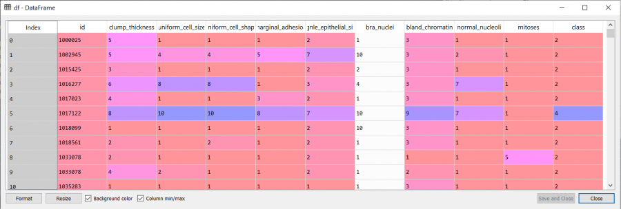
The names variable holds the 11 column labels. pd.read_csv reads .data files without complaint, and passing names to it labels the columns straight away. (pd is Pandas, remember.) After running that:

Looking at it

To check the size:

print(df.axes)
print (df.shape)

df.axes gives the number of rows and the column names. df.shape gives rows and columns. To reach a single row:

print(df.loc[0])
print(df.describe())

df.loc[0] through df.loc[698] print everything in that row. df.describe() gives you statistics like mean and standard deviation per column.

To see the distributions, use hist():

df.hist(figsize=(20,20))
plt.show()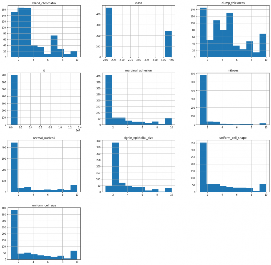

As the .names file said, every value in the table sits between 0 and 10. A scatter matrix is the other useful view:

scatter_matrix(df,figsize=(20,20))
plt.show()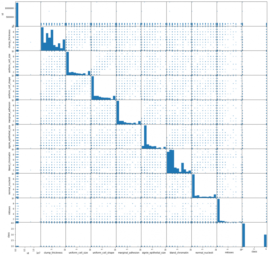

Training the classifier

Now we need train and test sets. You reach a column by name with df['class'], and class is the output we want, our Y. The inputs are the other 10 columns, so we drop class and feed what is left in as X.

X=np.array(df.drop(['class'],1))
y=np.array(df['class'])

Then split it: 80% of the data for training, 20% for testing. That is what test_size=0.2 means.

X_train,X_test,y_train,y_test=train_test_split(X,y,test_size=.2)

And build the SVM classifier:

mclf = svm.SVC(kernel='linear', C=1).fit(X_train, y_train)
print(clf.score(X_test, y_test))